Machine Learning Data Preprocessing, Splunk – Engine Data

Machine Learning Data Preprocessing for Splunk – Vibration Sensor Use Case

Machine learning data preprocessing is an essential prerequisite to training the ML model. Let’s consider a scenario where we employ machine learning to scrutinize data derived from an engine’s external vibration and internal speed sensors. The goal here is to predict potential malfunctions in the engine. You can customize this guide to fit any parameters or use cases you encounter while preparing data for machine learning. However, we will be using the vibration sensor as an example.

Affiliate: Experience limitless no-code automation, streamline your workflows, and effortlessly transfer data between apps with Make.com.

Steps to Take for Splunk Machine Learning Data Preprocess

First, we’ll do Data Collection and Preparation to gather the necessary data. We will need data from the external vibration sensor (x, y, z axis data) and the internal engine speed sensor. You can collect this data using Splunk’s data ingestion capabilities.

There are cases that after collecting the data, you’ll need to preprocess it. Machine learning data preprocessing might include cleaning the data and transforming it into a suitable format for a chosen ML algorithm. The field names that we will use:

external vibration sensor x-axis --> external_vib_x
external vibration sensor y-axis --> external_vib_y
external vibration sensor z-axis --> external_vib_z
internal engine speed sensor --> internal_speed

What is a Feature in Machine Learning

Machine learning is like teaching a computer to make educated guesses or predictions. But instead of using human intuition, the computer uses data. We call the pieces of data that the computer uses “features.” It is essential to understand your features while machine learning data preprocessing.

For instance, suppose you want to determine if an engine is running smoothly or having trouble. We could use these features:
1, 2, 3: A Vibration Sensor measures how much the engine is shaking in three directions: up/down (z-axis), left/right (x-axis), and forward/backward (y-axis). If the engine shakes significantly in either direction, it might indicate a problem.
4: An Internal Speed Sensor measures how fast the engine’s components move. If they’re moving too fast or too slow, that might also indicate a problem.

The computer takes these four features (the three vibration directions and the speed) and uses them to make its best guess about the engine’s condition. The more quality features we provide to the computer, the better its predictions can be.

Understanding and Visualizing Your Data Before Training the Machine Learning Model

Standardize the Data from the Vibration Sensor

You must decide what machine learning data preprocessing you need based on your data and the machine learning algorithm you choose.
We chose “KMeans,” an unsupervised machine learning algorithm part of the Machine Learning Toolkit (MLTK) for Splunk. Since we know only the good state of our engine and want to get alerted each time, there’s an anomaly from that state. The anomaly can be more or less vibrations or speed changes outside the good state range.

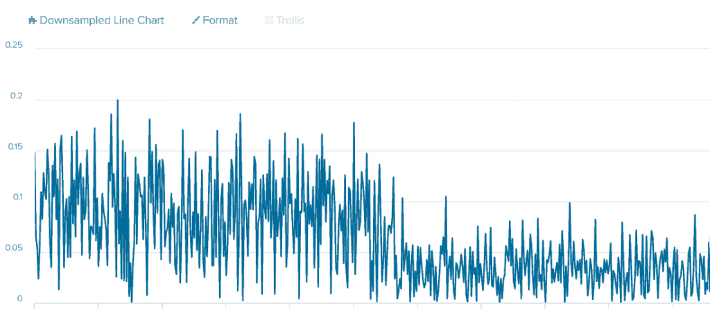
Look at the data:

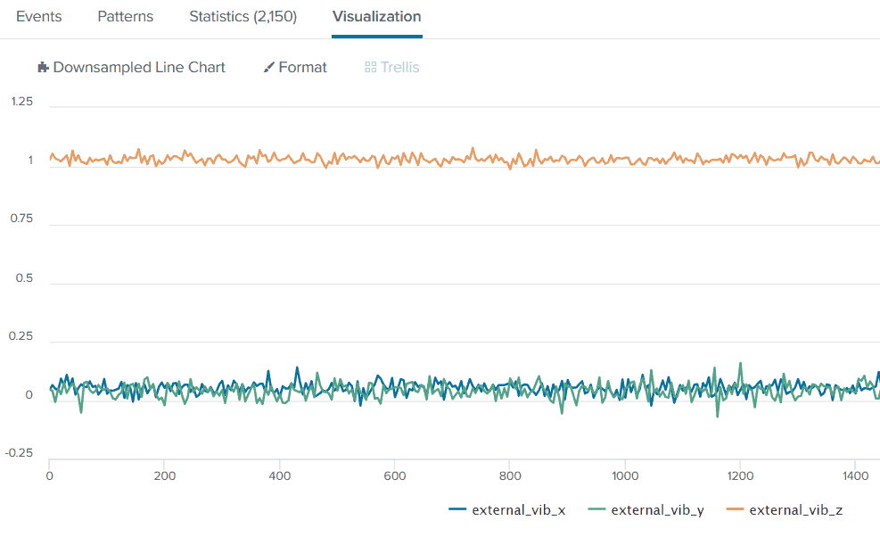
It is important to note that vibration sensors are different from one another, and each can output the three axes’ data differently. In our case, we see that X and Y axes center is slightly above “0,” and the z-axis data points center is way above “0”, around “1”, which is not the best scenario to use, so we’ll use standard scaling on the data set to center the data points to “0”. After that, we’ll consider applying a scaling of the points. There are two ways of applying standard scaling in Splunk: StandardScaler machine learning data preprocessing algorithm from Machine Learning Toolkit and built-in Splunk SPL commands to create appropriate variables and use them manually. Read about Standard Scaling and apply it in Splunk methods.

Since we will receive the data continuously from the sensor, using the StandardScaler algorithm from the Splunk Machine Learning Toolkit can be problematic because it is often applied to the whole set when future data points are known. So, we’ll be using built-in Splunk commands to apply standard scaling on data portions. You can read about it in the “Splunk Standard Scaling by Constant Interval” section of the Splunk Standard Scaling Preprocessing article.

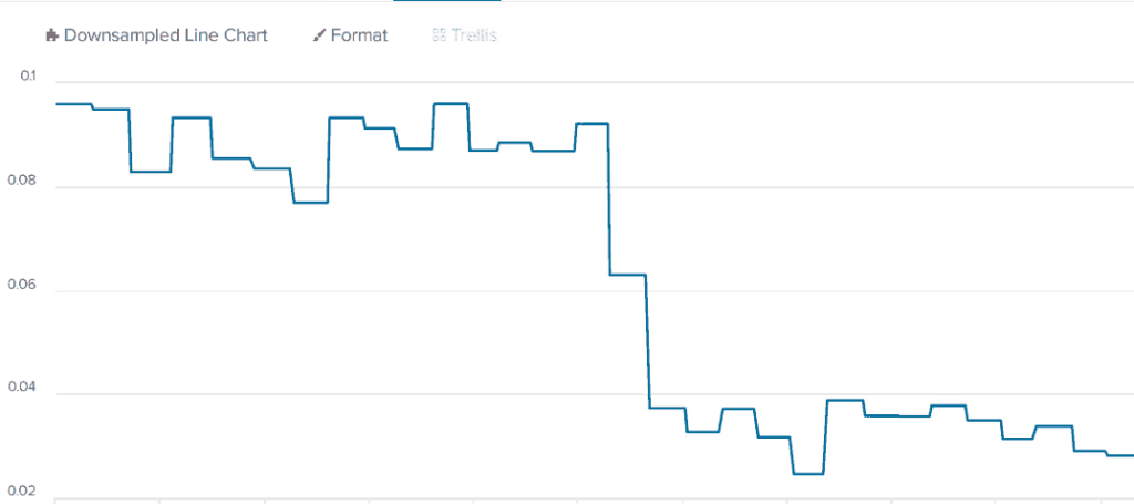
First, we’ll check how the algorithm will perform without data scaling but centering the data points only. Meaning we will use only the “mean” of each interval but not the standard deviation of the formula:

index=your_index
| bin _time span=15s as interval
| eventstats avg(external_vib_x) as mean_x, avg(external_vib_y) as mean_y, avg(external_vib_z) as mean_z by interval
| eval SS_x = (external_vib_x - mean_x), SS_y = (external_vib_y - mean_y), SS_z = (external_vib_z - mean_z)
| table _time SS_*
| sort _time

Your standardized data should look like this now:

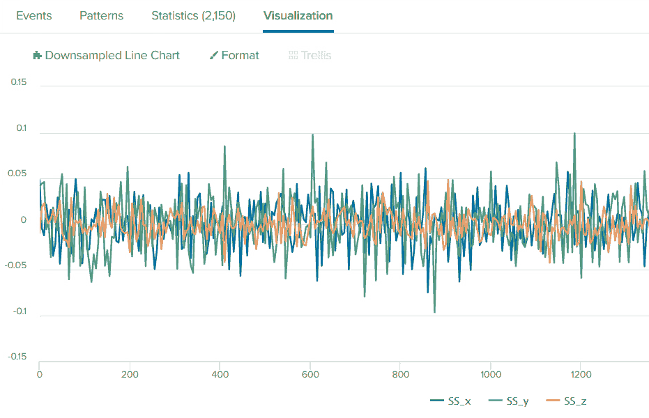
We can see that the center is at “0” now, and most of the data points have a similar scale besides “SS_y” having higher peaks. We’ll deal with that later. You can try adding the standard deviation variable to look at how your data change during machine learning data preprocessing:

index=your_index
| bin _time span=15s as interval
| eventstats avg(external_vib_x) as mean_x, stdev(external_vib_x) as stdev_x, avg(external_vib_y) as mean_y, stdev(external_vib_y) as stdev_y, avg(external_vib_z) as mean_z, stdev(external_vib_z) as stdev_z by interval
| eval SS_x = (external_vib_x - mean_x) / stdev_x, SS_y = (external_vib_y - mean_y) / stdev_y, SS_z = (external_vib_z - mean_z) / stdev_z

you will see that your maximum positive and negative scale on all the axes will be more proportional now. We’ll use averages later in our case. Hence, a more proportional scale was problematic because of the “KMeans” machine learning algorithm – the data points were very close for it to see the anomaly. So, we decided not to use the standard deviation variable in the standard scaling formula.

And this should be your practice, too, while machine learning data preprocessing and visualizing. If your chosen machine learning algorithm doesn’t work as you want, try changing how you preprocess data on different steps of the preprocessing stage and see how the ML algorithm reacts, which is very important for the optimal work of any algorithm.

As we pointed out in the Standard Scaling Normalization Preprocessing article (under “No Change in Input Data Will Result in a Standard Scaling of 0” header), you should note the static data on the Standard Scaling input, since it will result in “0” on the Standard Scaling output.

The Problem with Negative Numbers on Vibration Sensor Axes in KMeans Cluster Distance Calculations

To understand this situation, first, you need to grasp a couple of key concepts: What is KMeans, what does it mean by cluster distance, and how does a change in engine speed and vibration relate to all of this?

KMeans is a type of machine learning algorithm. The main usage of KMeans is for what’s called clustering. Imagine you’re looking at a scatter plot (a graph of dots). KMeans helps us to group those dots into clusters based on how close they are to each other. In the engine context, you can think of each dot as a state of the engine with certain properties like speed, vibration, and more.

Cluster distance is a measure of how far a dot is from the center of its cluster. The distance is small if a dot is right in the center of its cluster. If it’s on the edge, the distance is larger.

In our case, these “dots” are represented by engine vibrations on the axes. The measurement unit on each axis is “g.” The term “g” refers to the force exerted by gravity, which is used as a unit of measurement for acceleration and vibrations (on that a bit later). The vibration increases when the engine runs faster (around 0.2g or -0.2g). The vibration is lower when the engine runs slower (between 0.1g and -0.1g).

Before continuing with machine learning data preprocessing, we’ll explain the “g” metric.

The term “g” in the context of a vibration sensor stands for “gravity”. Specifically, it refers to “g-force,” a unit of acceleration caused by gravity.
The Earth’s gravity at sea level is approximately 9.81 m/s^2, often rounded to 10 m/s^2 for easier calculations, and is known as 1g.

When vibration sensors or accelerometers measure vibrations, they often use this “g” unit to express the magnitude of the vibrations. If a vibration sensor reads 2g, for example, it’s experiencing an acceleration twice that of Earth’s gravitational pull.
The above allows for an intuitive understanding of the forces involved, as we’re all familiar with the effects of Earth’s gravity on objects. It provides a standardized unit of measure that is easy to compare across different environments and applications.

Let’s understand the problem and why we need machine learning data preprocessing.
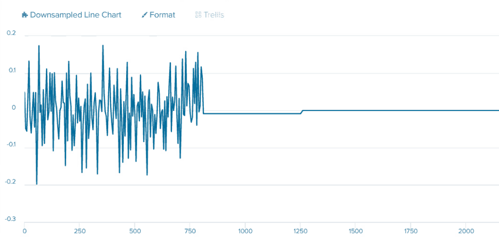
When training the KMeans model, you’ve set a good state (a normal working condition) with vibration acceleration between 0.2g and -0.2g. The KMeans algorithm calculated cluster distance for all the points. Now you have minimum and maximum cluster distance for all the points on the axes representing the normal working condition. If you slow down the engine, the vibration drops to 0.1g and -0.1g.
* The image shows an example only for one axis, which is similar behavior on all the axes.

You might expect that because the vibration is outside the range set for the good state, KMeans would flag it as an anomaly (something unusual). However, this isn’t the case.
Why not? Because, in this context, KMeans doesn’t simply look at whether the vibrations are between 0.2g and -0.2g. It looks at the cluster distances, i.e., how far the current vibration (the dot) is from the cluster’s center.

Even though the vibration has dropped to between 0.1g and -0.1g, it is still within the range of cluster distances that the KMeans algorithm considers part of the “good state” cluster distance, based on the training data. Therefore, it doesn’t view the reduced vibration as an anomaly.

On the other hand, if we trained the model at the speed when the vibration is at 0.2g and -0.2g and then made the engine move faster when the vibration on three axes would be around 0.3g to -0.3g, this would be definitely out of the normal cluster distance range that the algorithm set during training of the model. Because the amplitude of 0.3g to -0.3g is higher than the threshold set during training at 0.2g to -0.2g.

Convert Negative Numbers of Vibration Sensor Axes to Absolute Numbers as part of Machine Learning Data Preprocessing

To solve the problem, as the next step of machine learning data preprocessing, we will convert all the negative numbers on each axis of the vibration sensor to absolute numbers. Logically this is the right solution because positive and negative numbers on each axis symbolize the direction in which the engine is moving: up/down (z-axis), left/right (x-axis), and forward/backward (y-axis). The acceleration by which the engine is moving in each direction is the same. And what we are interested in is the measurement of the acceleration and not the direction. So, we can easily change the bi-directional data to one direction with absolute numbers. We will use the “abs” SPL command on standardized points on each axis:

| eval abs_external_vib_x=abs(SS_x), abs_external_vib_y=abs(SS_y), abs_external_vib_z=abs(SS_z)

In this command:
eval: This function allows you to create new fields using calculations, string manipulation, or assigning a value to a field.
abs: is a function that returns the absolute value of a number. The absolute value of a number is the number without its sign, so the absolute value of -2 is 2. The same is for a positive number; the absolute value of 2 is also 2. This command is useful for machine learning data preprocessing.
abs_external_vib_x=abs(SS_x), abs_external_vib_y=abs(SS_y), abs_external_vib_z=abs(SS_z): are creating new fields named “abs_external_vib_x”, “abs_external_vib_y”, and “abs_external_vib_z”. The value of these fields is the absolute value of the “SS_x,” “SS_y,” and “SS_z” fields in the data, respectively.

So, this command creates three new fields in your data: abs_external_vib_x, abs_external_vib_y, and abs_external_vib_z. Each field is the absolute value of the SS_x, SS_y, and SS_z fields.

Now we’ll add this to our full SPL command:

index=your_index
| bin _time span=15s as interval
| eventstats avg(external_vib_x) as mean_x, avg(external_vib_y) as mean_y, avg(external_vib_z) as mean_z by interval
| eval SS_x = (external_vib_x - mean_x), SS_y = (external_vib_y - mean_y), SS_z = (external_vib_z - mean_z)
| eval abs_external_vib_x=abs(SS_x), abs_external_vib_y=abs(SS_y), abs_external_vib_z=abs(SS_z)
| table _time abs_*
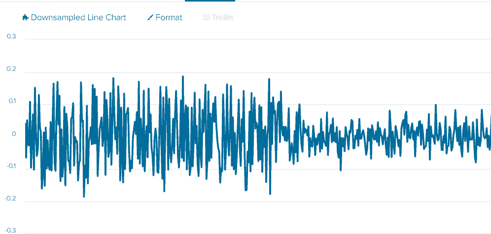
| sort _time

Showing only one axis for easier viewing:

The Average by Constant Time Intervals for Vibration Sensor Data

The image shows the engine’s minimum acceleration points at the normal working speed are near ~0g and a maximum of 0.2g. And if we look at the state when the engine speed is lower, and the maximum acceleration on this axis is 0.1g, we can also see that the minimum acceleration is also around 0g. This scenario still makes us a problem because the normal state during training with the threshold between ~0g and ~0.2g. When the engine speed and acceleration decreased to a range of ~0g to 0.1g, it was still within the normal state’s threshold.

We’ll use the next step in the machine learning data preprocessing stage to fix this issue. We will create an average of every 15 seconds of the vibration sensor data on each axis. This action will flatten all the minimum and maximum peaks of the data. If the training on normal engine operation data, the average was ~0.1g; then, during the engine section’s slower speed, the average will be ~0.05g, which is lower than during training and outside the normal threshold. The cluster distance KMeans will calculate for slower engine speed vibration will be outside the minimum and maximum cluster distance calculated for the normal operation state. Which you can understand will be an anomaly.

Splunk will calculate the average within the same 15-second bucket that we set for the “bin” command:

| eventstats avg(abs_external_vib_x) as avg_external_vib_x, avg(abs_external_vib_y) as avg_external_vib_y, avg(abs_external_vib_z) as avg_external_vib_z by interval

In this command:
eventstats is a Splunk command used to add summary statistics fields (like average, count, max, min, and more.) to all events, not just the final output, which means the calculated values are available for all subsequent commands in the pipeline, which is not the case with the “stats” command.
avg(abs_external_vib_x) as avg_external_vib_x, avg(abs_external_vib_y) as avg_external_vib_y, avg(abs_external_vib_z) as avg_external_vib_z is calculating the average value of three fields – abs_external_vib_x, abs_external_vib_y, and abs_external_vib_z – and renaming the result fields to avg_external_vib_x, avg_external_vib_y, and avg_external_vib_z, respectively. This command is another good example of machine learning data preprocessing.
by interval specifies that the averages should be calculated separately for each unique value of “interval” field. In our case, we set the one in with the “bin” command. In other words, it’s computing the average of abs_external_vib_x, abs_external_vib_y, and abs_external_vib_z at each distinct timestamp.

The outcome is that each event in your data will have three new fields, avg_external_vib_x, avg_external_vib_y, and avg_external_vib_z, which represent the average vibration in the x, y, and z directions absolute measurements, respectively, for the time associated with that event.

Adding that to the entire command:

index=your_index
| bin _time span=15s as interval
| eventstats avg(external_vib_x) as mean_x, avg(external_vib_y) as mean_y, avg(external_vib_z) as mean_z by interval
| eval SS_x = (external_vib_x - mean_x), SS_y = (external_vib_y - mean_y), SS_z = (external_vib_z - mean_z)
| eval abs_external_vib_x=abs(SS_x), abs_external_vib_y=abs(SS_y), abs_external_vib_z=abs(SS_z)
| eventstats avg(abs_external_vib_x) as avg_external_vib_x, avg(abs_external_vib_y) as avg_external_vib_y, avg(abs_external_vib_z) as avg_external_vib_z by interval
| table _time avg_*
| sort _time

Showing average for only one axis for easier viewing:

We used the “eventstats” command, adding processed value and new fields for each existing event in the database for each bucket of 15 seconds. You can execute that and see how it processes your data. You can use the “stats” command instead if you don’t want any other data points besides the averages. In this case, you will get only the average processed data points every 15 seconds.

Machine Learning Data Preprocessing – The Internal Speed Sensor Data

The KMeans algorithm is sensitive to significant differences between numbers in different features. For example, if we use only three features (the three axes of the vibration sensor) that have a scale between 0.00001 and 0.3, we will have calculated cluster distance for them between 0.001 and 0.000001. If we add a fourth feature with a range of 700 and 3000 (the engine speed in RPM), the cluster distance will change dramatically and can be around 700 to 2000. If we add to 700 the difference of 0.001 and 0.000001, we will get a range of 700.001 to 700.000001, which means that most weight during cluster distance calculation will be on speed change and not on vibration data. This scenario is problematic because we can tell that vibration sensor data is useless in this case. Each change in vibration will not do much of an effect on finding an anomaly in the engine operation. If the speed changes, you will see the anomaly in the calculated cluster distance out of the minimum and maximum cluster distance calculated during training. You might not see an anomaly when vibration data changes because it will be insignificant.

To overcome this, we will divide the internal sensor by 1000 to scale it down during the machine learning data preprocessing stage, so it will be closer to the vibration sensor axes scale:

| eval normal_internal_speed = internal_speed / 1000

Now internal speed will have a more proportional scale to axes data and more proportional weight in cluster distance calculations by the KMeans algorithm.

Full preprocessing command:

index=your_index
| bin _time span=15s as interval
| eventstats avg(external_vib_x) as mean_x, avg(external_vib_y) as mean_y, avg(external_vib_z) as mean_z by interval
| eval SS_x = (external_vib_x - mean_x), SS_y = (external_vib_y - mean_y), SS_z = (external_vib_z - mean_z)
| eval abs_external_vib_x=abs(SS_x), abs_external_vib_y=abs(SS_y), abs_external_vib_z=abs(SS_z)
| eventstats avg(abs_external_vib_x) as avg_external_vib_x, avg(abs_external_vib_y) as avg_external_vib_y, avg(abs_external_vib_z) as avg_external_vib_z by interval
| eval normal_internal_speed = internal_speed / 1000
| table _time avg_* normal_internal_speed
| sort _time

Reformat String Time that Came During Sampling of the Data

After creating the “bin” for the “interval” field and averaging with eventstats, the sorting wouldn’t work well since some time points would be missing. There are workarounds for this, but since we have a field called “sampled_time” that has the data in the format of “14:35:17.943200” (“%H:%M:%S.%f”) – we will use it. The problem is that the field is in string format, so we need to convert it to the timestamp in Splunk. Then, we can sort by this processed field and convert it to a human-readable format to understand it easily. We will not use this field in ML model training, so it is not part of the machine learning data preprocessing stage, but logically should be before or after that stage.

SPL solution:

| eval splunk_stime = strptime(sampled_time, "%H:%M:%S.%f")
| eval stime = strftime(splunk_stime, "%H:%M:%S.%f")

In this command:
| eval splunk_stime = strptime(sampled_time, “%H:%M:%S.%f”): This line takes the field “sampled_time” and converts it into epoch time (a way to track time as a running total of seconds) using the “strptime()” function. The “%H:%M:%S.%f” is the formatting string, which tells the function of how the “sampled_time” field is structured. In this case, it’s looking for hours (%H), minutes (%M), seconds (%S), and microseconds (%f).
| eval stime = strftime(splunk_stime, “%H:%M:%S.%f”): The second line takes the newly created epoch time field “splunk_stime” and converts it back into a string using the “strftime()” function. Again, “%H:%M:%S.%f” is the formatting string to convert the epoch time back into a string of hours, minutes, seconds, and microseconds.

Though “strftime” converts epoch time back to a string, without it, we could not sort by the “sampled_time” field. This problem can be due to data ingestion settings, so you might not have this problem if you have such a field.

Final SPL command:

index=your_index
| eval splunk_stime = strptime(sampled_time, "%H:%M:%S.%f")
| eval stime = strftime(splunk_stime, "%H:%M:%S.%f")
| bin _time span=15s as interval
| eventstats avg(external_vib_x) as mean_x, avg(external_vib_y) as mean_y, avg(external_vib_z) as mean_z by interval
| eval SS_x = (external_vib_x - mean_x), SS_y = (external_vib_y - mean_y), SS_z = (external_vib_z - mean_z)
| eval abs_external_vib_x=abs(SS_x), abs_external_vib_y=abs(SS_y), abs_external_vib_z=abs(SS_z)
| eventstats avg(abs_external_vib_x) as avg_external_vib_x, avg(abs_external_vib_y) as avg_external_vib_y, avg(abs_external_vib_z) as avg_external_vib_z by interval
| eval normal_internal_speed = internal_speed / 1000
| table _time stime avg_* normal_internal_speed
| sort stime

Since we need it only for sorting events by time during the application of the trained model, we will not use this during training.

Other Preprocessing Methods: Reduce the Number of Features by Using Vibration Sensor Axes Average

The above machine learning data preprocessing should get you started, but there are more methods you can use for preprocessing.
We have four features based on the fields we described: three axes of the external vibration sensor and internal engine sensor speed. You can create new features that can help improve the model. After applying the absolute numbers function to convert negative points to positives, you can calculate the average acceleration of the x, y, and z axes.

The SPL command:

| eval avg_total_vibration=(abs_external_vib_x+ abs_external_vib_y+ abs_external_vib_z)/3

In this command:
eval: This is the evaluation command in SPL. It allows you to calculate an expression and save the value into a field for each event.
avg_total_vibration=(abs_external_vib_x+ abs_external_vib_y+ abs_external_vib_z)/3: This part of the command is calculating a new field named “avg_total_vibration.” It does this by adding the values of three existing fields (abs_external_vib_x, abs_external_vib_y, and abs_external_vib_z) and dividing by 3. It calculates the average of these three fields for each event in your Splunk data – another technique for machine learning data preprocessing.

In simpler terms, the command adds the values of the three vibration sensors (x, y, and z) and divides the result by 3 to get the average. This average value, “avg_total_vibration,” represents the overall vibration sensed by the external sensors in three directions or dimensions.

It’s important to note that adding new features should be done wisely, as not all created features may improve the model’s performance. Though the fewer features the model has on its training input, the better it will work to analyze your data. Your machine learning model should perform better using only the average vibration data (one field) instead of three for the x, y, and z-axis fields. So, only two features will be on the input of machine learning model training: the three axes average of absolute data points and engine speed.

Other Preprocessing Methods: Use Simple Moving Average to Flatten the Peaks

It can be noisy when dealing with numerous vibration data, making it hard to identify patterns or trends. In this case, we can use Simple Moving Average (SMA), also suitable for machine learning data preprocessing.
Think of SMA as a way to smooth out your data. It’s a method where you calculate the average vibration reading over a certain period and then move this period step by step throughout your data.

Let’s say you’ve got these 10 data points from one of your vibration sensor’s axes:

[5, 8, 10, 13, 18, 20, 22, 24, 30, 33]

You now need to calculate a Simple Moving Average with a period of 4 (SMA4), which means you’ll calculate averages from sets of 4 consecutive numbers. Here’s how you do it:

(5 + 8 + 10 + 13) / 4 = 9
(8 + 10 + 13 + 18) / 4 = 12.25
(10 + 13 + 18 + 20) / 4 = 15.25
(13 + 18 + 20 + 22) / 4 = 18.25
(18 + 20 + 22 + 24) / 4 = 21
(20 + 22 + 24 + 30) / 4 = 24
(22 + 24 + 30 + 33) / 4 = 27.25

So, your SMA4 data set is now: [9, 12.25, 15.25, 18.25, 21, 24, 27.25]
Notice that we don’t have 10 points anymore. We have 7 points now. This effect happens because when we calculate moving averages, we lose some data points at the start due to the need for the initial set to calculate the average.
This SMA4 data set is smoother and less jumpy than your original data, which can help you identify trends and patterns more easily during machine learning data preprocessing.

Executing SMA4 with Splunk SPL:

| trendline sma4(abs_external_vib_x) as sma_external_vib_x, sma4(abs_external_vib_y) as sma_external_vib_y, sma4(abs_external_vib_z) as sma_external_vib_z
| fillnull value=0
| where sma_external_vib_x!=0 and sma_external_vib_y!=0 and sma_external_vib_z!=0
| table _time sma*
| sort _time

In this command:
We will execute SMA4 after we convert the negative numbers of each axis of the vibration sensor data to positives using the “abs” command. So, we’ll place the command we discussed after the “abs.”
trendline sma4(abs_external_vib_x) as sma_external_vib_x, sma4(abs_external_vib_y) as sma_external_vib_y, sma4(abs_external_vib_z) as sma_external_vib_z: The trendline command generates a statistical trendline function that operates on each time bucket in the data. It calculates a moving average (sma4, simple moving average of the last 4 data points) for three fields (abs_external_vib_x, abs_external_vib_y, abs_external_vib_z) and renames the output fields to sma_external_vib_x, sma_external_vib_y, and sma_external_vib_z, respectively.
fillnull value=0: This command fills null values in the data with zeros. Since we used sma4 to calculate SMA for the last 4 data points, the first 3 points will be empty, so we’ll be filling them with zeroes. You can fill it with anything you like or leave it as is without using the “fillnull” function. KMeans algorithm will not work with empty values, and you receive an error from Splunk after executing the “fit” command that there are empty values.
where sma_external_vib_x!=0 and sma_external_vib_y!=0 and sma_external_vib_z!=0: The “where” command filters the results based on the condition specified. In this case, it only allows events where the sma_external_vib_x, sma_external_vib_y, and sma_external_vib_z are not equal to zero. We now have the first three values as zeroes because we converted the empty values to zeroes with the “fillnull” command. Making KMeans train on zero data while you don’t have any in the SMA averages after that is not right, so we’re removing the rows with zero values. This command is also an important step in machine learning data preprocessing.
table _time sma*: The table command displays the specified fields in a tabular format. _time is the timestamp of each event, and sma* will display all fields starting with “sma.”
sort _time: This command sorts all events by the _time field in ascending order.

So, this script calculates a 4-point moving average on the absolute vibration data on the x, y, and z axes, fills any null values with zeros, filters out the data where the average is zero for any of the axes, displays the resulting time and averages in a table, and sorts the table in ascending order of time.

You can use any other integer rather than 4. If you want, you can use any different number, even SMA50, to make the trendline even smoother:

| trendline sma50(abs_external_vib_x) as sma_external_vib_x, sma50(abs_external_vib_y) as sma_external_vib_y, sma50(abs_external_vib_z) as sma_external_vib_z
| fillnull value=0
| where sma_external_vib_x!=0 and sma_external_vib_y!=0 and sma_external_vib_z!=0
| table _time sma*
| sort _time

Other Preprocessing Methods: Converting Strings to Numeric Data

KMeans algorithm doesn’t work with string data for its training input. But there are different machine learning data preprocessing techniques that you can use, like hashing your strings.

Splunk Essentials for Predictive Maintenance add-on

If you want additional help, you can use Splunk Essentials for Predictive Maintenance add-on. This add-on has more detailed examples of data ingestion, gathering, and preprocessing. It can help you more in your particular use case. In addition, it has a sample jet engine dataset on which you can practice Splunk machine-learning skills.